Pre-Trade Set-up – Pair Trading

Normal Distribution – Once Again

You must have read about the Normal Distribution in the Options module. If you haven’t, I would recommend you to go and read the chapter on Normal Distribution first.

This is a very important topic and it would be good for you to read that chapter before proceeding with this chapter. The concept of Normal Distribution is going to be used in both the pair trading techniques that we are going to discuss – Mark Wissler’s pair trading technique and the other technique that we will discuss later in the module.

Let me just briefly repeat the concept of Normal Distribution once again to refresh your memory.

General concept of Normal distribution that you should know –

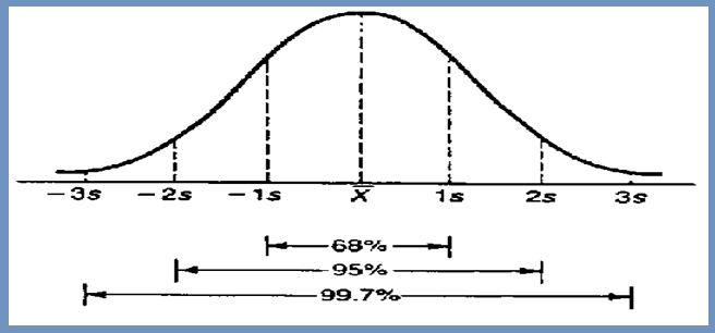
Within 1st standard deviation you can see 68% of data

Within 2nd standard deviation you can see 95% of data

Within 3rd standard deviation you can see 99.7% of data

You can also see these points as below image

 

Well, for your information, let me tell you that data is distributed in many ways, such as uniform distribution, binomial distribution, exponential distribution, etc.

Statistical Distribution

In the previous chapter, we discussed three parameters related to statistics – mean, median and mode. Now we will calculate these three for paired data, that is, we will find the mean, median and mode for difference, spread and ratio. We will do this work through an Excel sheet.

I will continue working on the Excel sheet that I worked on in the previous chapter. If you want, you can download this Excel sheet through the link given at the end of the chapter.

This sheet has been set up in this way

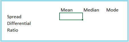
Excel functions are

Mean – ‘=average()’
Median – ‘=median()’
Mode – ‘=mode.mult()’
The numbers are given below –

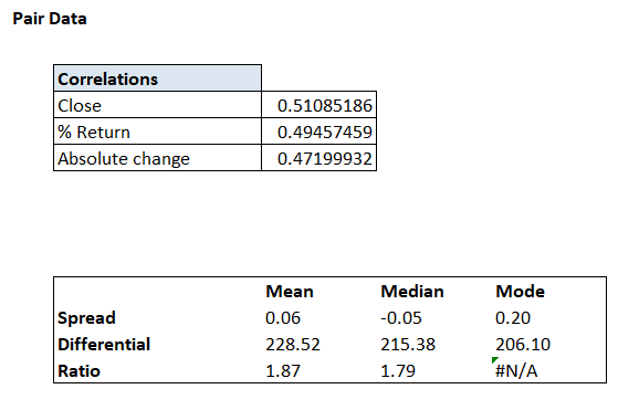
As you can see, the correlation numbers were calculated in the previous chapter itself.

Now our data set up is ready, now we have to add only one variable here which is – standard deviation. The concept of standard deviation has been explained to you earlier.

Standard deviation shows the distance or change from the average i.e. deviation. The definition given in the books of standard deviation is – “In statistics, standard deviation (SD from the Greek word sigma σ) is a measure that tells how much change or variation or dispersion has occurred in a given data.”

So in a way, standard deviation tells us how much change is taking place in the data i.e. how much is its variability, which tells us how much the data is spread. Now I try to explain it in the context of my pair of data.

Here is the differential data we extracted some time back –

In total, we have 496 difference data points. We calculated the average of these a little earlier in this chapter, which is 228.52.

Now if I ask you, how much variation does this data point show from the mean, i.e., how much variability does it have? Or, put another way, why do I need to know how far this data point shows from the mean, i.e., how much variability does it have?

In fact, if we don’t know how far our data can move from the mean, it will be difficult for us to assess the behavior of that data. For example, when we get the 498th data point, we will be able to see whether the data is around the mean or within a range.

In fact, this is the most important thing in pair trading.

The way to measure this variation is the standard deviation.

Personally, I think standard deviation is the easiest way to measure it, but there are many traders who use another method called absolute deviation. Both standard deviation and absolute deviation tell us about the changes that can happen in the data. But both of these look at the data in different ways.

While I was looking for a way to explain the difference between standard deviation and absolute deviation, I came across an explanation on Investopedia that I really liked, so I am giving it here –

There can be many ways to measure the changes that can happen in any data set, but the two most popular methods are standard deviation and average deviation. Both of these are quite similar but there is some difference in the way they are calculated and the way they are drawn. Finding range and volatility are considered very important in the world of finance, so people associated with accounting, investing and economics have to understand both of them well.

Standard deviation is the most common way to measure variability in data. It is often used to measure volatility in the stock market and other investments. To find or calculate standard deviation, first you have to find the variance. For this, you have to subtract the mean from each data point, then find its square, add them together and then find the average of all these. By the way, variance in itself is a good way to find variability and range. The higher the variance, the greater the spread of the data. Standard deviation is actually nothing but the square root of the variance. Squaring the difference between each data point and the mean is good because it avoids the negative difference that comes from data points below the mean. But this also means that the units of variance are different from the units of the actual data. Hence, the square root of the variance is taken so that the standard deviation can be brought back to the actual units and it is easier to use and draw conclusions from it.

Another way to measure variability is the average deviation, also known as the absolute deviation. The actual data is used as is to calculate the average deviation. The numbers are not squared here to avoid the problem of negative difference between the data and the mean. To calculate the average deviation, the mean is subtracted from each data point, then all of them are added, and then the average is calculated. In this method, the mean absolute value is used less because taking the absolute value makes the further calculations bigger and more difficult than using the standard deviation.

Now we will find standard deviation and absolute deviation for all three components of pair data – mean, median and mode.

I have made a change here – I have kept the Y-Axis for mean, median and mode and the X-Axis for difference ratio and spread. Because of this there will be a slight difference between the picture above and the picture below.

Excel functions to find these variables are

Standard Deviation – ‘=Stdev.p()’

Absolute Deviation – ‘=avedev()’

One more thing – Mean, Median, Mode, Standard Deviation and Absolute Deviation are also known as Basic Descriptive Statistics.

Standard Deviation Table

As you know that standard deviation tells us how much variation or change is taking place in the data. Now let us go a little further and try to measure this variation or change. By doing this we will know how much variation or change is seen from the mean number. For example, the 498th difference data can be 275. By measuring the variation, we can find out whether 275 is above the mean or very much below the mean.

Based on this information, we can decide whether we should buy the pair or we should short the pair. By the way, we will discuss this later. But for now, let us try to measure the variation. To do this, we first need to create a table called the standard deviation table.

This table looks like this

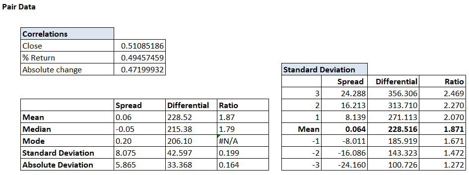
Now we will find the value of 1st, 2nd and 3rd standard deviation above the mean and below the mean for spread difference and ratio.

Let us first focus on the spread data. The mean of the spread is 0.06. We also know that the standard deviation is 8.075.

So, the 1st standard deviation above the mean is

0.064 + 8.075 = 8.139

2nd SD –

0.064 + (2*8.075) = 16.123

3rd SD –

0.064 + (3*8.075) = 24.288

These are all the values ​​above the mean. Similarly, we can find the values ​​below the mean as well.

-1 SD –

0.064 – 8.075 = -8.011

-2 SD –

0.064 – (2*8.075) = -16.086

-3 SD –

0.064 – (3*8.075) = -24.160

I have done these calculations for the differential and ratio as well, and the table now looks like this –

If the 498th difference data shows a number of 315 then we can very quickly deduce that it is near +2 standard deviations and with 95% confidence we can say that the next data point has only a 5% chance of being above 315.

So at the moment we have all the data that can help us draw conclusions about the pair and tell if there is an opportunity to trade there or not. In the next chapter we will go ahead and do just that.

Key points from this chapter

• Normal distribution plays a very important role in pair trading
• 68% of the data is captured in the 1st standard deviation
• 95% of the data is captured in the 2nd standard deviation
• 99.7% of the data is captured in the 3rd standard deviation
• Standard deviation and absolute deviation are used to measure the variation in the data
• The standard deviation table allows us to compare the current data with the expected variation.
• The standard deviation table gives us an indication of whether we should go long or short in a pair trade

“At Gaurav Heera Academy, we take pride in being the best in providing stock market courses in Delhi. With expert mentorship, practical training, and a proven track record, we ensure our students gain the skills needed to succeed in the stock market. Join us today and take your trading journey to the next level!”